MATLAB:Plotting
This page will primarily go over some examples of different ways to plot data sets.
Using Different Line Styles
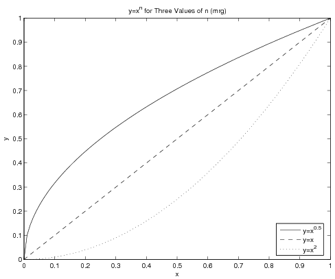
Most of the time, you will be plotting three or fewer different lines on a single window, and they can thus be distinguished from one another in MATLAB by using different line styles. There are two different ways to get multiple data sets plotted in the same figure - use the hold on...hold off paradigm or pu all the "plot triplets" in a single plot command. What follows is an example of the latter case:
x = linspace(0, 1, 100);
y1 = x.^0.5;
y2 = x.^1;
y3 = x.^2;
plot(x, y1, 'k-', x, y2, 'k--', x, y3, 'k:');
legend('y=x^{0.5}', 'y=x', 'y=x^2', 0);
title('y=x^n for Three Values of n (mrg)');
xlabel('x');
ylabel('y');
print -deps CurvePlot % note that adds .eps to filename
The figure this creates will be:
Note the legend - the use of the final argument 0 will make MATLAB look for the best spot in the window for the legend - which is to say, somewhere not conflicting with any of the lines if at all possible. Also note that the text in the legend and in the title contains basic LaTeX code for obtaining the superscripts.
Using Different Point Styles
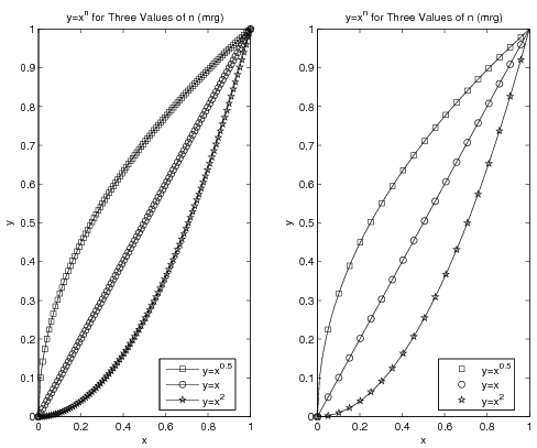
Sometimes there will be more data sets on a graph than there are line styles in MATLAB. In cases like this, you may think to use symbols at the points. The problem with that becomes clear if you have a large number of data points - you do not want to try to jam hundreds of symbols onto a curve. The left graph in the figure below shows what a disaster that could be. Instead, you can plot a line with all your data but plot points on top of the line with only some of the data. The right side of the figure shows the result of this operation. The code for both graphs in the figure is given below it.
x = linspace(0, 1, 100);
y1 = x.^0.5;
y2 = x.^1;
y3 = x.^2;
subplot(1,2,1) % left graph (ewwwwwww)
plot(x, y1, 'k-s', x, y2, 'k-o', x, y3, 'k-p');
legend('y=x^{0.5}', 'y=x', 'y=x^2', 0);
title('y=x^n for Three Values of n (mrg)');
xlabel('x');
ylabel('y');

subplot(1,2,2) % right graph (ooo.  aah.  wow)
plot(x, y1, 'k-', x, y2, 'k-', x, y3, 'k-'); % lines only!
incr = 5;
hold on % hols lines and now add points
PointPlot=plot(...
    x(1:incr:end), y1(1:incr:end), 'ks',...
    x(1:incr:end), y2(1:incr:end), 'ko',...
    x(1:incr:end), y3(1:incr:end), 'kp');
hold off
legend(PointPlot, 'y=x^{0.5}', 'y=x', 'y=x^2', 0);
title('y=x^n for Three Values of n (mrg)');
xlabel('x');
ylabel('y');
Note that the assignment of one of the plots to the variable PointPlot is required so that the legend can be told which set of
plots to use as a basis for the legend. Without this, it would be
possible for the legend to be based on the plot using solid lines (which are
the same for all three data sets) rather than to be based on the
plot using the symbols.

