Symbolic/Examples/Circuits

Brute Force 1

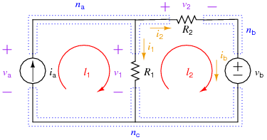
The following example shows the "brute force" method of setting up and solving for all the element currents and voltages for a simple resistive circuit and then using those solutions to solve for auxiliary information (in this case, some powers). The circuit involved is:

Equations

Element Equations

Mainly, these are Ohm's Law equations for the resistors, so:

\( \begin{align} R_1:& & v_1&=i_1R_1\\ R_2:& & v_2&=i_2R_2 \end{align} \)

KCL Equations

The number of independent KCL equations s one less than the number of nodes, so in this case, 2. Note: all three nodal KCL equations are written below, but node \(n_c\)'s is not used in the Maple worksheet.

\( \begin{align} KCL,n_a:& & -i_a+i_1+i_2&=0\\ KCL,n_b:& & -i_2+i_b&=0\\ KCL,n_c:& & i_a-i_1-i_b&=0 \end{align} \)

KVL Equations

The number of independent KVL equations is equal to the number of meshes for a 2-D circuit, or to the number of elements, minus the number of nodes, plus one for circuits in general. In this case, that is 2 independent KVL (two meshes, or 3 elements - 3 nodes + 1 = 2). For the brute force method, just use the mesh equations:

\( \begin{align} KVL,l_1:& & -v_a+v_1&=0\\ KVL,l_2:& & -v_1+v_2+v_b&=0 \end{align} \)

Auxiliary Equations

For this example, the auxiliary equations will be used to determine the power delivered by each source and the power absorbed by each resistor:

\( \begin{align} p_{del,i_a}&=v_ai_a & p_{del,v_b}&=-v_bi_b \\ p_{abs,R_1}&=v_1i_1 & p_{abs,R_2}&=v_2i_2 \end{align} \)

Note that all elements except for \(i_a\) are labeled passively.

Code

Maple

The Maple worksheet for this example is available for download: Circuit1Demo.mw. You can also look at a PDF of the code. The code assumes that:

\( \begin{align} R_1&=1000~\Omega & R_2&=2200~\Omega\\ i_a&=0.005~\mbox{A} & v_b&=12~\mbox{V} \end{align} \)

There are also versions of the file that show how you can use Maple's built-in ability to use units, which are accessed via the Units menu on the left side of the screen. The code for this example is available for download: Circuit1DemoUnits.mw. You can also look at a PDF of the code. Note that using units works seamlessly for some applications but becomes very cumbersome in others (especially once differential equations or transforms are involved).

The file is also available on the Maple Cloud. You can view the worksheet even if you do not have Maple; if you have Maple, you can download the worksheet and edit it. Maple Cloud Link

Python

Starting in 2022, we are looking at using Python to perform symbolic calculations. This demo is still in beta!