ECE 280/PlotDemo

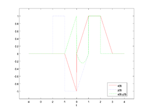
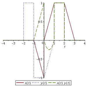
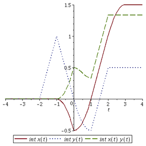
The following is a demonstration of how to perform similar tasks in Maple and MATLAB. Specifically, this example shows how to define the unit step and ramp functions, use them to define accumulated signals, create functions to calculate the integrals of those signals, and plot both the signals and their integrals. The comments are meant to show the different sections of each piece of code. The resulting figures are connected with each particular program.

MATLAB

Code

% MATLAB and Maple Demo
% M. R. Gustafson II

%% Initialize
clear

%% Define step and ramp functions
ustep = @(in) (1.0).*(in>=0);
uramp = @(in)  (in).*(in>=0);

%% Define x and y using accumulation
X = @(t) (-1)*uramp(t+1)+ustep(t)+(2)*uramp(t)+(-1)*uramp(t-1)+(-1)*uramp(t-2)+(1)*uramp(t-3);
Y = @(t) ustep(t+2)+(-2)*ustep(t+1)+uramp(t)+(-1)*uramp(t-1)+ustep(t-1)-ustep(t-2);

%% Plot signals
t = linspace(-4, 4, 1e4);
figure(1); clf
plot(t, X(t), 'r-', ...
     t, Y(t), 'b:', ...
     t, X(t).*Y(t), 'g--')
legend('x(t)', 'y(t)', 'x(t) y(t)', 'location','best')
xlabel('t')
gzoom

%% Calculate integrals
IntX  = @(t) cumtrapz(t, X(t));
IntY  = @(t) cumtrapz(t, Y(t));
IntXY = @(t) cumtrapz(t, X(t).*Y(t));

%% Plot integrals
figure(2); clf
plot(t, IntX(t), 'r-', ...
     t, IntY(t), 'b:', ...
     t, IntXY(t), 'g--')
legend('\int x(t)', '\int y(t)', '\int x(t) y(t)', 'location','best')
xlabel('t')
gzoom

%% Save plots (not in Maple)
figure(1); print -dpng SignalPlot
figure(2); print -dpng IntegralPlot

xMaple

Note - for the xMaple code, if you copy and paste it, all the code will go in one execution group (thus the ; at the end of each line). I haven't figured out the smart way to put things in multiple lines...

# Maple and MATLAB Demo
# M. R. Gustafson II
# Initialize
restart;
# Define step and ramp functions
U := t-> Heaviside(t); 
R := t->  t*U(t); 
# Define x and y using accumulation
X := t->  -R(t+1)+U(t)+2*R(t)-R(t-1)-R(t-2)+R(t-3); 
Y := t->  U(t+2)-2*U(t+1)+R(t)-R(t-1)+U(t-1)-U(t-2); 
# Plot signals
plot([X(t), Y(t), X(t)*Y(t)], t = -4 .. 4, linestyle = [1, 2, 3], legend = ['x(t)', 'y(t)', 'x(t)*y(t)']);
# Calculate integrals
IntX := t->  int(X(tau), tau = -infinity .. t);
IntY := t->  int(Y(tau), tau = -infinity .. t);
IntXY := t->  int(X(tau)*Y(tau), tau = -infinity .. t);
# Plot integrals
plot([IntX(t), IntY(t), IntXY(t)], t = -4 .. 4, linestyle = [1, 2, 3], legend = ['int*x(t)', 'int*y(t)', 'int*x(t)*y(t)']);

Plots

MATLAB

xMaple