Difference between revisions of "ECE 280/Fall 2021/HW 02"
Jump to navigation
Jump to search
(→Using MATLAB) |
|||
| (One intermediate revision by the same user not shown) | |||
| Line 4: | Line 4: | ||
There are a few options when it comes to using MATLAB: | There are a few options when it comes to using MATLAB: | ||
* You can install it for free on your own computer - see [[MATLAB#Installation]] | * You can install it for free on your own computer - see [[MATLAB#Installation]] | ||
| − | * You can use MATLAB Online once you have a MathWorks account associated with Duke. You will need to go through the first part of the [https://oit.duke.edu/help/articles/kb0023255#matlab1 MATLAB at Duke] page to get the account set up. Once that is done, go to [https://matlab.mathworks.com/ MATLAB Online] and log in with your MathWorks credentials. Note that all your files will be on the MATLAB cloud; | + | * You can use MATLAB Online once you have a MathWorks account associated with Duke. You will need to go through the first part of the [https://oit.duke.edu/help/articles/kb0023255#matlab1 MATLAB at Duke] page to get the account set up. Once that is done, go to [https://matlab.mathworks.com/ MATLAB Online] and log in with your MathWorks credentials. Note that all your files will be on the MATLAB cloud; to access them directly from your computer, install the [https://www.mathworks.com/products/matlab-drive.html MATLAB Drive Connector] |
| − | to access them directly from your computer, install the [https://www.mathworks.com/products/matlab-drive.html MATLAB Drive Connector] | ||
| − | |||
* You could use MATLAB in a Duke Container but this is currently MATLAB R2014a and will not work with Simulink so...it's a no go for now. | * You could use MATLAB in a Duke Container but this is currently MATLAB R2014a and will not work with Simulink so...it's a no go for now. | ||
Latest revision as of 19:30, 6 September 2021
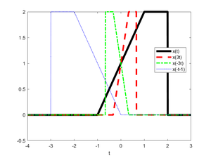
This page is meant as a support page for HW 02. The codes and graphs are for zyBook Challenge Activity 1.2.3
Contents
Using MATLAB and Python
Using MATLAB
There are a few options when it comes to using MATLAB:
- You can install it for free on your own computer - see MATLAB#Installation
- You can use MATLAB Online once you have a MathWorks account associated with Duke. You will need to go through the first part of the MATLAB at Duke page to get the account set up. Once that is done, go to MATLAB Online and log in with your MathWorks credentials. Note that all your files will be on the MATLAB cloud; to access them directly from your computer, install the MATLAB Drive Connector
- You could use MATLAB in a Duke Container but this is currently MATLAB R2014a and will not work with Simulink so...it's a no go for now.
Using Python
I generally recommend using Anaconda for Python, and specifically using the Spyder IDE. You can download Anaconda at the Individual Edition Download link. To start Python:
- Windows:
- Go to the Start menu -> Anaconda3 -> Spyder, or
- Go to the Start menu -> Anadonda3 -> Anaconda Navigator and the click Spyder, or if those don't work,
- Go to the Start menu -> Anaconda3 -> Anaconda prompt and then when it comes up type
spyderand hit return
- macOS:
- Search for Anaconda, start Anaconda Navigator and the click Spyder, or if that doesn't work,
- Search for
terminal, start a terminal, and then when it comes up typespyderand hit return
Turning The Assignment In
For this assignment, you will be attaching 8 files:
- The MATLAB code (text files ending in .m) for 1.2.11 and 1.4.11
- The MATLAB graphs (in .png format) for 1.2.11 and 1.4.11
- The Python code (text files ending in .py) for 1.2.11 and 1.4.11
- The Python graphs (in .png format) for 1.2.11 and 1.4.11
Make sure the names of the Python graphs are different from the names of the MATLAB graphs! Yuo will upload all eight things to the HW 2 Part 3 assignment in gradescope.
MATLAB
 1 %% Initialize workspace
 2 clear
 3
 4
 5 %% Define singularity functions
 6 u = @(t) (t>=0)*1;
 7 r = @(t) t.*u(t);
 8
 9 %% Define x(t)
10 x = @(t) r(t+1) - r(t-1) - 2*u(t-2);
11
12 %% Create time base
13 t = linspace(-4, 3, 1000);
14
15 %% Initialize figure
16 figure(1)
17 clf
18
19 %% Make plots
20 plot(t, x(t), 'k-', 'linewidth', 4), hold on
21 plot(t, x(3*t), 'r--', 'linewidth', 3)
22 plot(t, x(-3*t), 'g-.', 'linewidth', 2)
23 plot(t, x(-t-1), 'b:', 'linewidth', 1), hold off
24
25 %% Add label and legend
26 xlabel('t')
27 legend('x(t)', 'x(3t)', 'x(-3t)', 'x(-t-1)', 'location', 'best')
28
29 %% Save figure
30 print -dpng CA010203matlab_plot
Python
 1 # %% Import modules
 2 import numpy as np
 3 import matplotlib.pyplot as plt
 4
 5 # %% Define singularity functions
 6 u = lambda t: (t>=0)*1
 7 r = lambda t: t*u(t)
 8
 9 # %% Define x(t)
10 x = lambda t: r(t+1) - r(t-1) - 2*u(t-2)
11
12 # %% Create time base
13 t = np.linspace(-4, 3, 1000)
14
15 # %% Initialize figure and axes
16 fig = plt.figure(num=1, clear=True)
17 ax = fig.add_subplot(1, 1, 1)
18
19 # %% Make plots
20 ax.plot(t, x(t), 'k-', linewidth=4)
21 ax.plot(t, x(3*t), 'r--', linewidth=3)
22 ax.plot(t, x(-3*t), 'g-.', linewidth=2)
23 ax.plot(t, x(-t-1), 'b:', linewidth=1)
24
25 # %% Add label and legend
26 ax.set(xlabel='t')
27 ax.legend(['x(t)', 'x(3t)', 'x(-3t)', 'x(-t-1)'], loc='best')
28
29 # %% Save figure
30 fig.tight_layout()
31 fig.savefig("CA010203python_plot.png")

