ECE 280/Examples/Convolution

The following is an example of convolving two signals; the convolution is done several different ways:

1. Math... So much math.
2. Using Convolution Shortcuts
3. Geometrically, flipping and shifting \(h(t)\)
4. Geometrically, flipping and shifting \(x(t)\)

Setup

The goal for this problem is to determine the output \(y(t)\) created by an input \(x(t)\) for a linear time invariant system if the system's impulse response \(h(t)\) is known. In this particular example:

\( \begin{align} x(t)&=2u(t)-u(t-1)-u(t-3)\\ h(t)&=e^{-t}u(t)\\ y(t)&=x(t)*h(t)=\int_{-\infty}^{\infty}x(\tau)h(t-\tau)d\tau=\int_{-\infty}^{\infty}x(t-\tau)h(\tau)d\tau \end{align} \)

where the particular choice of which integral to use is up to the user.

Math

Given the relative complexity of \(x(t)\), it may make more sense to use the first form, where \(h(t)\) is flipped and shifted. That yields:

\( \begin{align} y(t)&=\int_{-\infty}^{\infty}x(\tau)h(t-\tau)d\tau\\ y(t)&=\int_{-\infty}^{\infty}\left(2u(\tau)-u(\tau-1)-u(\tau-3)\right)\left(e^{-(t-\tau)}u(t-\tau)\right)d\tau \end{align} \)

Distributing terms gives:

\( \begin{align} y(t)&=\int_{-\infty}^{\infty}2e^{-(t-\tau)}u(\tau)u(t-\tau)d\tau\dots\\ ~&~-\int_{-\infty}^{\infty}e^{-(t-\tau)}u(\tau-1)u(t-\tau)d\tau\dots\\ ~&~-\int_{-\infty}^{\infty}e^{-(t-\tau)}u(\tau-3)u(t-\tau)d\tau\\ \end{align} \)

Taking the first part alone:

\( \int_{-\infty}^{\infty}{\color{Brown}2e^{-(t-\tau)}}{\color{Red}u(\tau)}{\color{Blue}u(t-\tau)}d\tau \)

note that the integrand is only non-zero when two conditions are met simultaneously:

\( \begin{align} {\color{Red}0}&{\color{Red}<\tau} & {\color{Blue}\tau}&{\color{Blue}<t} \end{align} \)

Furthermore, those conditions can only be met simultaneously if the outer conditions are met; that is, if:

\( \begin{align} {\color{Purple}0}&{\color{Purple}<t} \end{align} \)

These three conditions lead to three changes. The limits on \(\tau\) change the limits of the integral with respect to \(\tau\) while the condition on \(t\) can be represented by a unit step of \(t\). In other words:

\( \begin{align} \int_{-\infty}^{\infty}{\color{Brown}2e^{-(t-\tau)}}{\color{Red}u(\tau)}{\color{Blue}u(t-\tau)}d\tau &= {\color{Purple}u(t)}\int_{{\color{Red}0}}^{{\color{Blue}t}}{\color{Brown}2e^{-(t-\tau)}}d\tau\\ {\color{Purple}u(t)}\int_{{\color{Red}0}}^{{\color{Blue}t}}{\color{Brown}2e^{-(t-\tau)}}d\tau&= u(t)\left[2e^{-(t-\tau)} \right]_0^{t}=\left(2-2e^{-t}\right)u(t) \end{align} \)

Note with that last line that the integral is with respect to \(\tau\) and the exponent of \(\tau\) is +1. The other two components of the convolution integral can be processed in a similar way:

\( \begin{align} \int_{-\infty}^{\infty}{\color{Brown}-e^{-(t-\tau)}}{\color{Red}u(\tau-1)}{\color{Blue}u(t-\tau)}d\tau &= {\color{Purple}u(t-1)}\int_{{\color{Red}1}}^{{\color{Blue}t}}{\color{Brown}-e^{-(t-\tau)}}d\tau\\ {\color{Purple}u(t-1)}\int_{{\color{Red}1}}^{{\color{Blue}t}}{\color{Brown}-e^{-(t-\tau)}}d\tau&= -u(t-1)\left[e^{-(t-\tau)} \right]_1^{t}=-\left(1-1e^{-(t-1)}\right)u(t-1) \end{align} \)

and

\( \begin{align} \int_{-\infty}^{\infty}{\color{Brown}-e^{-(t-\tau)}}{\color{Red}u(\tau-3)}{\color{Blue}u(t-\tau)}d\tau &= {\color{Purple}u(t-3)}\int_{{\color{Red}3}}^{{\color{Blue}t}}{\color{Brown}-e^{-(t-\tau)}}d\tau\\ {\color{Purple}u(t-3)}\int_{{\color{Red}3}}^{{\color{Blue}t}}{\color{Brown}-e^{-(t-\tau)}}d\tau&= -u(t-3)\left[e^{-(t-\tau)} \right]_3^{t}=-\left(1-1e^{-(t-3)}\right)u(t-3) \end{align} \)

meaning (finally) that:

\( \begin{align} y(t)=x(t)*h(t)=\left(2-2e^{-t}\right)u(t)-\left(1-1e^{-(t-1)}\right)u(t-1)-\left(1-1e^{-(t-3)}\right)u(t-3) \end{align} \)

Written piecewise, this equation would be:

\( \begin{align} y(t)&=\begin{cases} {\color{Black}0} & {\color{Black}t<0} \\ 2-2e^{-t} & {\color{Black}0<t<1}\\ 1 - 2e^{-t}+ e^{-(t-1)} & {\color{Black}1<t<3}\\ -2e^{-t} + e^{-(t-1)} + e^{-(t-3)} & {\color{Black}t>3} \end{cases} \end{align} \)

Shortcuts

Full color version:

To use the shortcuts, first distribute the various components of the convolution:

\( \begin{align} x(t)&=\color{Brown}{2u(t)-u(t-1)-u(t-3)}\\ h(t)&=\color{Blue}{e^{-t}u(t)}\\ x(t)*h(t)&=\color{Brown}{2u(t)}*\color{Blue}{e^{-t}u(t)}\color{Brown}{-u(t-1)}*\color{Blue}{e^{-t}u(t)}\color{Brown}{-u(t-3)}*\color{Blue}{e^{-t}u(t)} \end{align} \)

These can be rearranged, pulling out any shifts, as:

\( \begin{align} x(t)*h(t)&=\color{Orange}{2}\color{Blue}{e^{-t}u(t)}*\color{Red}{u(t)}\color{Orange}{-}\color{Blue}{e^{-t}u(t)}*\color{Red}{u(t)}\color{Orange}{*\delta(t-1)}\color{Orange}{-}\color{Blue}{e^{-t}u(t)}*\color{Red}{u(t)}\color{Orange}{*\delta(t-3)} \end{align} \)

Note that each component now has a convolution of

\( \begin{align} \color{Blue}{e^{-t}u(t)}*\color{Red}{u(t)} \end{align} \)

in it. Convolution with a step generates an integral, and integrating the right-sided exponential yields:

\( \begin{align} \color{Red}{\int_{-\infty}^{t}}\color{Blue}{e^{-\tau}u(\tau)}d\tau=u(t)\left[-e^{-\tau}\right]_0^t=\color{Fuchsia}{(1-e^{-t})u(t)} \end{align} \)

which means the rearranged functions can be re-written as:

\( \begin{align} x(t)*h(t)&=\color{Orange}{2}\color{Fuchsia}{(1-e^{-t})u(t)}\color{Orange}{-}\color{Fuchsia}{(1-e^{-t})u(t)}\color{Orange}{*\delta(t-1)}\color{Orange}{-}\color{Fuchsia}{(1-e^{-t})u(t)}\color{Orange}{*\delta(t-3)} \end{align} \)

Now the shifts can be applied to give:

\( \begin{align} x(t)*h(t)&=2(1-e^{-t})u(t)-(1-e^{-(t-1)})u(t-1)-(1-e^{-(t-3)})u(t-3) \end{align} \)

Black and white only:

To use the shortcuts, first distribute the various components of the convolution:

\( \begin{align} x(t)&={\color{Black}2u(t)-u(t-1)-u(t-3)}\\ h(t)&={\color{Black}e^{-t}u(t)}\\ x(t)*h(t)&={\color{Black}2u(t)}*{\color{Black}e^{-t}u(t)}{\color{Black}-u(t-1)}*{\color{Black}e^{-t}u(t)}{\color{Black}-u(t-3)}*{\color{Black}e^{-t}u(t)} \end{align} \)

These can be rearranged, pulling out any shifts, as:

\( \begin{align} x(t)*h(t)&={\color{Black}2}{\color{Black}e^{-t}u(t)}*{\color{Black}u(t)}{\color{Black}-}{\color{Black}e^{-t}u(t)}*{\color{Black}u(t)}{\color{Black}*\delta(t-1)}{\color{Black}-}{\color{Black}e^{-t}u(t)}*{\color{Black}u(t)}{\color{Black}*\delta(t-3)} \end{align} \)

Note that each component now has a convolution of

\( \begin{align} {\color{Black}e^{-t}u(t)}*{\color{Black}u(t)} \end{align} \)

in it. Convolution with a step generates an integral, and integrating the right-sided exponential yields:

\( \begin{align} {\color{Black}\int_{-\infty}^{t}}{\color{Black}e^{-\tau}u(\tau)}d\tau=u(t)\left[-e^{-\tau}\right]_0^t={\color{Black}(1-e^{-t})u(t)} \end{align} \)

which means the rearranged functions can be re-written as:

\( \begin{align} x(t)*h(t)&={\color{Black}2}{\color{Black}(1-e^{-t})u(t)}{\color{Black}-}{\color{Black}(1-e^{-t})u(t)}{\color{Black}*\delta(t-1)}{\color{Black}-}{\color{Black}(1-e^{-t})u(t)}{\color{Black}*\delta(t-3)} \end{align} \)

Now the shifts can be applied to give:

\( \begin{align} x(t)*h(t)&=2(1-e^{-t})u(t)-(1-e^{-(t-1)})u(t-1)-(1-e^{-(t-3)})u(t-3) \end{align} \)

Geometrically Flipping/Shifting \(h\)

The geometric method involves determining the piecewise regions in \(\tau\) where the different functions overlap as a function of \(t\). With the current example, the only change \(h(t)\) makes is at \(t=0\), while \(x(t)\) has four different parts. The piecewise definitions of the two functions can be written as:

\( \begin{align} x(t)&= \begin{cases} 0 & t<0 \\ 2 & 0<t<1 \\ 1 & 1<t<3 \\ 0 & t>3\end{cases} & h(t)&= \begin{cases} 0 & t<0 \\ e^{-t} & t>0\end{cases} & \end{align} \)

In the convolution integral

\( \begin{align} y(t)&=x(t)*h(t)=\int_{-\infty}^{\infty}x(\tau)h(t-\tau)d\tau \end{align} \)

the piecewise definitions of the signals change to functions of \(\tau\):

\( \begin{align} x(\tau)&= \begin{cases} 0 & \tau<0 \\ 2 & 0<\tau<1 \\ 1 & 1<\tau<3 \\ 0 & t>3\end{cases} & h(t-\tau)&= \begin{cases} e^{-(t-\tau)} & \tau<t \\ 0 & \tau>t\end{cases} \end{align} \)

As \(t\) changes, \(x(\tau)\) does not move but \(h(t-\tau)\) does, resulting in different components of the two functions overlapping at different times. The following four subsections will show what happens as \(t\) increases.

t<0

Before overlap

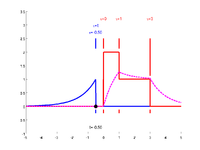
The "leading edge" of \(h(t-\tau)\) is at \(\tau=t\); until \(t>0\), there will be no overlap with \(x(\tau)\) and thus the convolution integral will be 0:

\( \begin{align} y(t)&=\begin{cases} {\color{Black}0} & {\color{Black}t<0} \end{cases} \end{align} \)

0<t<1

First overlap

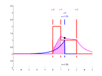
Once \(t>0\), the segment of \(h\) that is nonzero passes into the region of \(x\) that is equal to the constant 2. This will remain the situation until \(h\)'s transition into the region where \(x\) is 1. During this phase, the integrand will be the product of the exponential from \(h\) and the 2 from \(x\):

\( \begin{align} y(t)&=\begin{cases} {\color{Black}0} & {\color{Black}t<0} \\ {\color{Black}\int_{{\color{Red}0}}^{{\color{Blue}t}}{\color{Red}2}{\color{Blue}e^{-(t-\tau)}}~d\tau} & {\color{Black}0<t<1} \end{cases} \end{align} \)

1<t<3

Second overlap

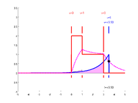
After \(t>1\) but before \(t>3\), there are two different regions of overlap: the region where \(x\) is 2 now overlaps for \(0<\tau<1\) while the region where \(x\) is 1 overlaps where \(1<\tau<t\). That yields:

\( \begin{align} y(t)&=\begin{cases} {\color{Black}0} & {\color{Black}t<0} \\ {\color{Black}\int_{{\color{Red}0}}^{{\color{Blue}t}}{\color{Red}2}{\color{Blue}e^{-(t-\tau)}}~d\tau} & {\color{Black}0<t<1}\\ {\color{Black}\int_{{\color{Red}0}}^{{\color{Red}1}}{\color{Red}2}{\color{Blue}e^{-(t-\tau)}}~d\tau} + {\color{Black}\int_{{\color{Red}1}}^{{\color{Blue}t}}{\color{Red}1}{\color{Blue}e^{-(t-\tau)}}~d\tau} & {\color{Black}1<t<3} \end{cases} \end{align} \)

t>3

Final overlap

Finally, once \(t>3\), the leading edge of the flipped \(h\) has passed the edge of \(x\) and the limits of integration are thus purely dependent on the piecewise boundaries of \(x\) alone:

\( \begin{align} y(t)&=\begin{cases} {\color{Black}0} & {\color{Black}t<0} \\ {\color{Black}\int_{{\color{Red}0}}^{{\color{Blue}t}}{\color{Red}2}{\color{Blue}e^{-(t-\tau)}}~d\tau} & {\color{Black}0<t<1}\\ {\color{Black}\int_{{\color{Red}0}}^{{\color{Red}1}}{\color{Red}2}{\color{Blue}e^{-(t-\tau)}}~d\tau} + {\color{Black}\int_{{\color{Red}1}}^{{\color{Blue}t}}{\color{Red}1}{\color{Blue}e^{-(t-\tau)}}~d\tau} & {\color{Black}1<t<3}\\ {\color{Black}\int_{{\color{Red}0}}^{{\color{Red}1}}{\color{Red}2}{\color{Blue}e^{-(t-\tau)}}~d\tau} + {\color{Black}\int_{{\color{Red}1}}^{{\color{Red}3}}{\color{Red}1}{\color{Blue}e^{-(t-\tau)}}~d\tau} & {\color{Black}t>3} \end{cases} \end{align} \)

After Integration

After calculating all those integrals, the answer would be:

\( \begin{align} y(t)&=\begin{cases} {\color{Black}0} & {\color{Black}t<0} \\ 2-2e^{-t} & {\color{Black}0<t<1}\\ (2e^{-(t-1)}-2e^{-t})+(1-e^{-(t-1)}) & {\color{Black}1<t<3}\\ (2e^{-(t-1)}-2e^{-t}) + (e^{-(t-3)}-e^{-(t-1)})& {\color{Black}t>3} \end{cases} \end{align} \)

or, combined,

\( \begin{align} y(t)&=\begin{cases} {\color{Black}0} & {\color{Black}t<0} \\ 2-2e^{-t} & {\color{Black}0<t<1}\\ 1 - 2e^{-t}+ e^{-(t-1)} & {\color{Black}1<t<3}\\ -2e^{-t} + e^{-(t-1)} + e^{-(t-3)} & {\color{Black}t>3} \end{cases} \end{align} \)

Geometrically Flipping/Shifting x

The geometric method involves determining the piecewise regions in \(\tau\) where the different functions overlap as a function of \(t\). With the current example, the only change $h(t)$ makes is at \(t=0\), while \(x(t)\) has four different parts. The piecewise definitions of the two functions can be written as:

\( \begin{align} x(t)&= \begin{cases} 0 & t<0 \\ 2 & 0<t<1 \\ 1 & 1<t<3 \\ 0 & t>3\end{cases} & h(t)&= \begin{cases} 0 & t<0 \\ e^{-t} & t>0\end{cases} & \end{align} \)

In the convolution integral

\( \begin{align} y(t)&=x(t)*h(t)=\int_{-\infty}^{\infty}x(t-\tau)h(t)d\tau \end{align} \)

the piecewise definitions of the signals change to functions of \(\tau\):

\( \begin{align} x(t-\tau)&= \begin{cases} 0 & \tau<t-3 \\ 1 & t-3<\tau<t-1 \\ 2 & t-1<\tau<0 \\ 0 & \tau>3\end{cases} & h(\tau)&= \begin{cases} 0 & \tau<0 \\ e^{-\tau} & \tau>0\end{cases} \end{align} \)

As \(t\) changes, \(h(\tau)\) does not move but \(x(t-\tau)\) does, resulting in different components of the two functions overlapping at different times. The following four subsections will show what happens as \(t\) increases.

t<0

Before overlap

The "leading edge" of \(x(t-\tau)\) is at \(\tau=t\); until \(t>0\), there will be no overlap with \(h(\tau)\) and thus the convolution integral will be 0:

\( \begin{align} y(t)&=\begin{cases} {\color{Black}0} & {\color{Black}t<0} \end{cases} \end{align} \)

0<t<1

First overlap

Once \(t>0\), the segment of \(x\) that is equal to the constant 2 passes into the region of \(h\) that is non-zero. This will remain the situation until \(x\)'s transition to the constant 1 passes into that region. During this phase, the integrand will be the product of the exponential from \(h\) and the 2 from \(x\):

\( \begin{align} y(t)&=\begin{cases} {\color{Black}0} & {\color{Black}t<0} \\ {\color{Black}\int_{{\color{Blue}0}}^{{\color{Red}t}}{\color{Red}2}{\color{Blue}e^{-\tau}}~d\tau} & {\color{Black}0<t<1} \end{cases} \end{align} \)

1<t<3

Second overlap

After \(t>1\) but before \(t>3\), there are two different regions of overlap: the region where \(x\) is 1 now overlaps for \(0<\tau<t-1\) while the region where \(x\) is 2 overlaps where \(t-1<\tau<t-3\). That yields:

\( \begin{align} y(t)&=\begin{cases} {\color{Black}0} & {\color{Black}t<0} \\ {\color{Black}\int_{{\color{Blue}0}}^{{\color{Red}t}}{\color{Red}2}{\color{Blue}e^{-\tau}}~d\tau} & {\color{Black}0<t<1} \\ {\color{Black}\int_{{\color{Blue}0}}^{{\color{Red}t-1}}{\color{Red}1}{\color{Blue}e^{-\tau}}~d\tau} + {\color{Black}\int_{{\color{Red}t-1}}^{{\color{Red}t}}{\color{Red}2}{\color{Blue}e^{-\tau}}~d\tau} & {\color{Black}1<t<3} \end{cases} \end{align} \)

t>3

Final overlap

Finally, once \(t>3\), the trailing edge of the flipped \(x\) has passed the edge of \(h\) and the limits of integration are thus purely dependent on the piecewise boundaries of \(x\) alone:

\( \begin{align} y(t)&=\begin{cases} {\color{Black}0} & {\color{Black}t<0} \\ {\color{Black}\int_{{\color{Blue}0}}^{{\color{Red}t}}{\color{Red}2}{\color{Blue}e^{-\tau}}~d\tau} & {\color{Black}0<t<1} \\ {\color{Black}\int_{{\color{Blue}0}}^{{\color{Red}t-1}}{\color{Red}1}{\color{Blue}e^{-\tau}}~d\tau} + {\color{Black}\int_{{\color{Red}t-1}}^{{\color{Red}t}}{\color{Red}2}{\color{Blue}e^{-\tau}}~d\tau} & {\color{Black}1<t<3}\\ {\color{Black}\int_{{\color{Red}t-3}}^{{\color{Red}t-1}}{\color{Red}1}{\color{Blue}e^{-\tau}}~d\tau} + {\color{Black}\int_{{\color{Red}t-1}}^{{\color{Red}t}}{\color{Red}2}{\color{Blue}e^{-\tau}}~d\tau} & {\color{Black}t>3} \end{cases} \end{align} \)

Animation of Flipped/Shifted x

Coming soon!

External References

• Erik Cheever's [Convolve GUI] for MATLAB - an excellent way to visualize convolution using MATLAB